Having a good teacher can change your life. When I was in high-school, I ended up enrolled in a theoretical maths class thought by an older man called Roger. This didn't go very well. In fact, I was failing. Hard to say why, for sure, but I know that I didn't study much or care about maths at this time. But I loved Roger's classes. And I loved Roger. He was open, funny, knowledgeable in the best ways, and a great teacher overall. It was clear that he loved maths and wanted to share his passion with us. This was the reason that I stayed. And because I stayed for so long, he actually took me aside one day and asked me to switch to a simpler class, if I wanted to graduate at all. Looking back today, it's obvious that I was inspired by Roger, but I don't think we were the best teacher-student combo. I have been thinking more about this recently, about what it means to be a good student and teacher.

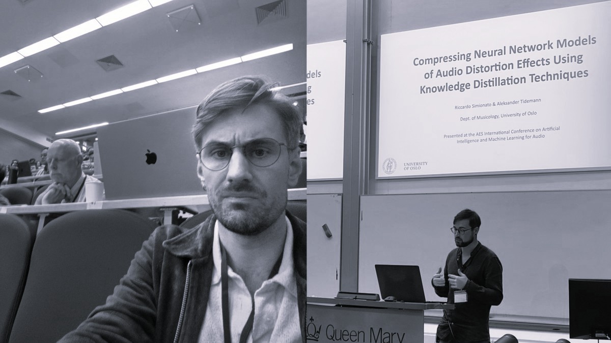
I am currently in a hot and crowded conference room at Queen Mary University College in London, listening to a talk about AI ethics at the first-ever international conference on AI and Machine Learning for Audio, hosted by the Audio Engineering Society in September 2025 (called AES AIMLA). I am here because me and my friend and former colleague Riccardo Simionato are presenting our latest research on compression techniques for neural audio effects. It all started last spring, when Riccardo asked me if I wanted to help him explore whether we could make neural audio effects, which are audio effects built with neural networks, smaller and more efficient using a compression technique called knowledge distillation. With knowledge distillation, features from large neural networks, called teachers, are essentially transferred or distilled to smaller networks, called student. So essentially, a good student-teacher combo.

Back in the conference room, the question in the air is about AI and how it will affect the music industry. An older gentleman man just raised his hand and confidently signaled the speaker. Through a long comment, the man argued that we might better understand the fate of AI in the music industry by looking to other similar technological advancements that have occured in the past, like MP3. Online sharing and MP3 were thought to be the end of the music industry as we knew it and there was a lot of criticism and concern about piracy, especially. Of course the music industry changed a lot during this time, but MP3's role in the matter was less significant than expected. Quick side-note, I later learned that the guy commenting actually was a central character in the development of the original MP3 codec, sometime in the 80s and 90s. His comment also reminded me of a graph I saw recently that depicted how the popularity of new technologies almost always tends to receede over time, that our expectations are almost always wrong. Might this be the case with AI as well? Are we currently at the very peak of the curve, waiting for the imminent fall? I don't know what the fate of AI will be, of course, nor do I think the MP3-man has all the answers.

But what I certainly do feel is that it's hard to find good teachers in life, regardless of whether you're a high-school student, a reseracher at an AI conference, or a neural network tying to be a better and smaller version of yourself. And just finding a good teacher is rarely enough. You have to find someone, or something, that fits you and your current situation well.

In this post, I will take on the role as a teacher and try to present to you, my student, our AES paper on knowledge distillation for neural audio effects in the best way possible. The post touches on central concepts in virtual-analog modeling and digital compression techniques, but focuses mainly on our experiments and findings. Before you start, you can also check our our full AES research paper from here, or see the GitHub repository with source code and plugin/VST versions of our distortion models. Finally, if you just want to hear how our models sound, you can also jump straight to some audio examples here.

Virtual-analog modeling and audio effects compression

It was not too long ago that researchers in the field of Virtual-Analog (VA) modeling discovered how effective it was to use neural networks to digitally emulate analog audio effects. The advantages of using machine learning for VA-modeling are many, but it comes down to its exceptional ability to find patterns in large quantities of data. Analog audio effects consist of complex hardware circuits that shape the sound in an unpredictable and non-linear way. These non-linearities are hard to describe mathematically. With machine learning, however, we can essentially skip the hard part and train models to recreate the analog behaviour without us actually knowing intricate inner goings on. This approach, of treating the analog audio effect as a "black box", is amply called black-box modeling. The process concerned with mathematically describing the details in the hardware circuitry is called white-box modeling.

Black-box approaches to modeling audio effects have been successful on a wide variety of effects, including tube amplification, distortion, optical compressors, and other time-based effects. This has been possible using certain neural architectures, particularly Convolutional Neural Networks (CNN) and Recurrent Neural Networks (RNN). But one major issue is that these networks can easily become large and clunky, requiring significant amounts of operations per sample during runtime. This is a problem because we usually want audio effects to be computationally efficient and run smoothly on many consumer-grade devices, like laptops and phones. Said in another way, large neural networks can hinder the real-time capabilities of models that strive for efficiency. We want our neural audio effects to be as lightweight as possible.

But making neural audio effects smaller, i.e reducing the number of operations in the network, is hard and often harmful to the quality and accuracy of models (how good they sound). But despite the challenges, many compression techniques exist that are able to optimize the size of neural network models without compromising too much on performance. For instance, Pruning is a technique that identifies and removes parameters in a neural networks that seem redundant and therefore contributes less to the training process. Pruning has been shown to be effective on RNN networks of audio effects. There is also Quantization, a technique that compresses networks by lowering the bits required to represent each weight of the network, and Low-rank factorization, which uses matrix and tensor decomposition to identify redundant weights, all of which have been proven to be effective compression methods for neural audio effects.

Finally, there is knowledge distillation.

Distilling the knowledge of neural audio effects

Knowledge distillation (KD) is a technique where smaller neural networks, often called students, are trained to mimic a larger teacher network. This works by leveraging the fact that neural networks capture meaningful and complex representations of their training data in hidden layers of their networks. Once a teacher network achieves good generalization and performance on a set of data, its knowledge can be transferred to a smaller student network through the process called distillation. Read more about the inner workings of KD on neural networks, check out this famous paper by Geoffrey Hinton et al.

What was interesting to us about KD, scientifically speaking, was that this technique had not been explored for neural audio effects before. In fact, we found very few cases where KD was applied to regression problems at all (which is what is used when handling real-time audio), and none dealing with audio distortion effects. The bulk of existing research on KD with audio is mostly concerned with classification tasks.

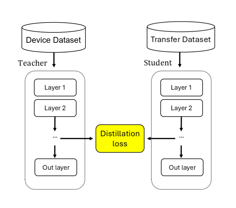
There are three primary types of KD for neural networks, each with a unique approach to the distillation process. We have response-based, feature-based, and relation-based KD. For our experiments, we choose to focus on feature-based distillation. If you're interested in learning more about these other types of KD, I recommend this blog post. In short, instead of teaching students to mimic the output of a teacher model, feature-based KD focuses on transferring, or distilling, a teacher's internal representations, or features, to a smaller student network, as seen in Figure 1. The idea is that this "feature transplant" allows student models to capture more nuanced representations of the input data, leading to improved generalization and performance.

Additionally, with feature-based distillation, specific layers of the teacher network are identified as important intermediary feature representations of the input data. Similar intermediate layers of a student network are then aligned to those of the teacher. During training, the student model learns to produce feature maps similar to the teacher model, inheriting its structure and hierarchical understanding of the data. To make the model learn, a loss function is defined to minimize the difference between the feature representations of the teacher and student models at these corresponding layers, as illustrated in Figure 1 above.

Building and training our distortion VST network

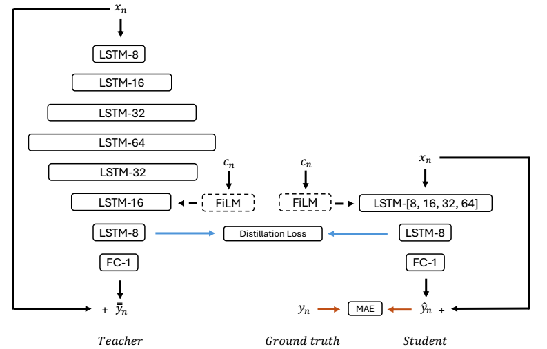
To experiment with KD on audio distortion effects, we first built a general neural network architecture using recurrent LSTMs. This approach has become a common starting point for modeling neural audio effects of this sort. The goal of our experiments was not only to see whether KD was successful on neural audio effects, but also to examine and learn more about the relationship between teacher and student models. What configuration works best, and why? To explore this, we experimented with slightly different network architectures for both the teacher and student models, each with varying network depths and sizes.

For teachers, we opted for two different configurations; one large with seven hidden layers and units distributed in an hourglass shape, as shown in Figure 2, and one smaller with only two hidden layers with fixed unit sizes. All our student models consisted also of two hidden layers, but each with a varying number of units in the second layer. In total, we tried four different student configurations per teacher model, varying the unit size in the second layer from 8 to 64.

No two distortion units sound the same, especially not analog ones. It's because of this that using more than one dataset can be wise to get a better idea about how your models are working. For our training and evaluation, we used data from three different audio distortion devices: the Blackstar HT-1 vacuum tube amplifier, Electro-Harmonix Big Muff guitar pedal, and the analog-modeled overdrive VST plugin DrDrive. The datasets themselves consisted of a bunch of 10-minute-long audio files where the distortion effects were added to various music, such as frequency sweeps, white noise, physical recordings of bass, drums, piano, pads and sections from various pop/rock songs. The HT-1 and Big Muff data was sourced from previous research projects (Südholt 2023, Wright 2019), but we collected the DrDrive data ourselves using DGMD, a standalone software for generating datasets for audio-related ML tasks (Fasciani 2023). You can also read more about the DGMD software project in a previous post of mine.

We also had time to experiment with some conditioned data. The primary difference between conditioned and unconditioned datasets is that conditioned data (sometimes referred to as parametric data) includes one or more parameters that add additional dimensions to the dataset. Because making models perform well on both conditioned and unconditioned data is very challenging, and therefore interesting, we wanted to include at least one conditioned case in our evaluation. When dealing with audio effects, conditioning is usually represented in the form of added effect parameters, such as Drive, Brightness, Dry/Wet, Amplitude, etc. In the end, we included a conditioned version of the DrDrive dataset in our evaluation with one parameter, the 'Drive' knob, which determines the amount of distortion applied to the input signal. This made four datasets in total for our evaluation.

For both students and teachers, our training strategy was to run each model 1000 epochs. An early stopping mechanism was in place to stop training if there was no reduction in validation loss for 30 consecutive epochs. The batch size is set to 8 examples, with each example composed of 2048 input audio samples. You can read much more in-depth descriptions about the training strategy, loss function (MAE), and other evaluation metrics in the full paper.

Results and key takeaways

Overall, the results from our experiments were positive, showing that Knowledge distillation has the potential to improve the performance of neural audio effects. But the interesting part is how they improve performance, and to what degree.

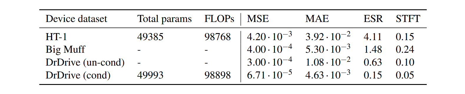
Table 1 presents the test loss results of the large hourglass-shaped teacher models, while Table 2 displays the performance of both distilled and non-distilled student models. Distilled students are those taught by a larger teacher network, and non-distilled students are the standard ones trained on the regular dataset. The way to read these tables is to compare the distilled and non-distilled loss metrics of students with the same network architecture (the S-8-16 markings, and so on). If a distilled student shows a lower loss score than its non-distilled counterpart, then that model is performing better. The key here is to realize that these models are the same exact size. So, if a distilled student performs better than a non-distilled student for a given network, it means that we could (in theory) reduce the size of the distilled model and still achieve the same performance as the non-distilled one. This is how we know that our knowledge distillation is working.

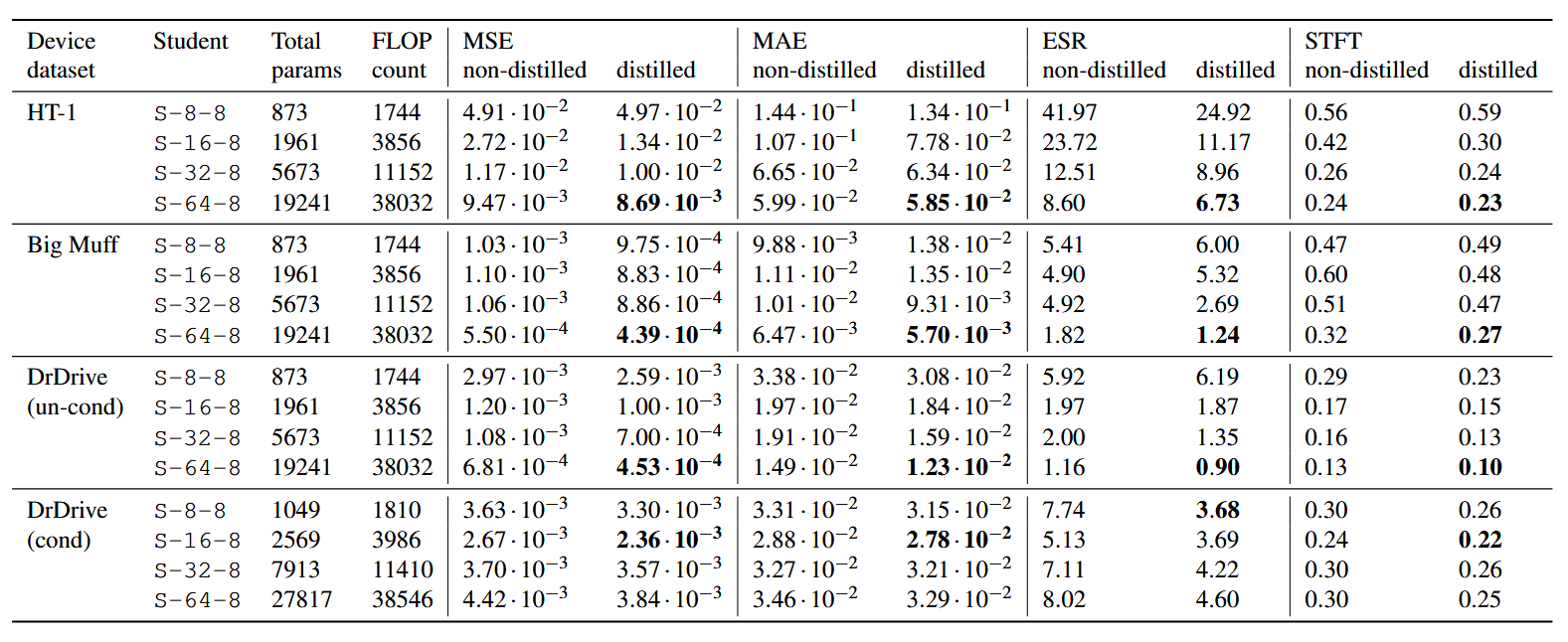
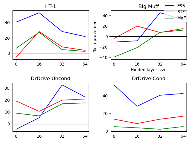
The results tell us that student models typically performed better with larger hidden layer sizes (units). This suggests that the effectiveness of distillation is proportional to the size of the models. Figure 3 takes a closer look at this. Here, the size of the second student LSTM layers are represented along the X-axis, while the improvement of using distilled models over non-distilled models is detailed along the Y-axis (in %). So, a high score on the Y-axis means that there is a big performance advantage in favor of using the distilled model for that particular unit size. Graphing this paints a clearer picture of how distillation seems to improve as the size of the student models increases. However, some metrics tell another story. For instance, the ESR loss exhibits large variability, with both extreme negative and positive values. This variance could be caused by ESR being a normalized function, and that the distillation improves more when the signal's amplitude is larger than low.

Also, the HT-1 and the conditioned set of DrDrive seem to improve more at lower model sizes. Some of the smallest student models (8 units) even show negative improvements from distillation. This is particularly true with Big Muff and the unconditioned set of DrDrive. However, these two both seem to recover quickly at 16 units and beyond, following an upward trend, like the rest. It's also noteworthy that when non-distilled students are performing well, the benefits of distillation are much less pronounced.

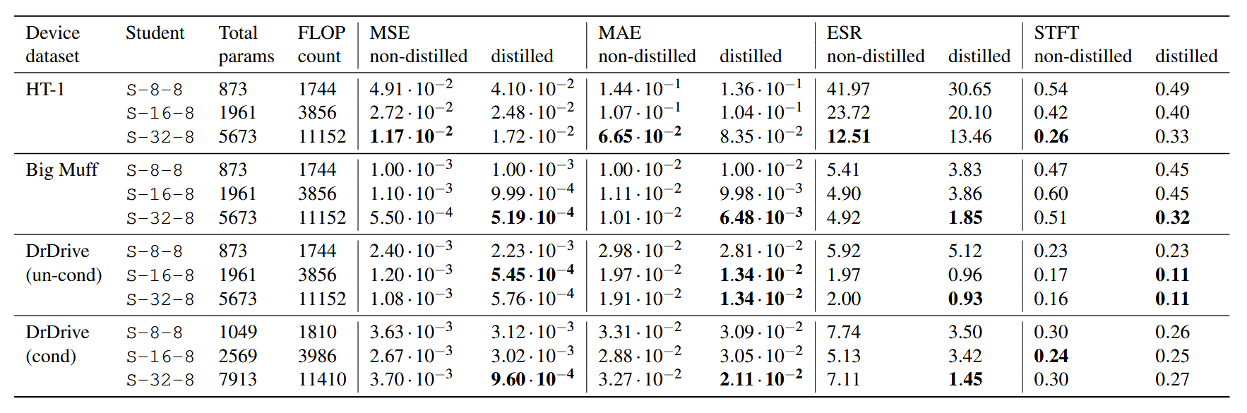
Further, it's not conclusive from the results which teacher architecture is best for any given student. But we did observe that the smallest teacher model (with only two layers) was more effective than the large hourglass-shaped teacher when it came to the smallest students. In this scenario, the complexity gap is smaller between the teacher and the student. This might be a hint. These results are presented in Table 3, below.

Listening tests

In addition to the quantitative results, we conducted a MUSHRA-style listening test to explore the perceptual quality of distilled versus non-distilled models. Does one sound better than the other? And if so, in what way? Our hypothesis was that distilled models would sound better than non-distilled models with the same unit size, matching the quantitative results.

In each listening test trial, participants were subjected to five audio examples and one reference example of the distortion units applied to either guitar, bass, or drum signals. The audio examples included both distilled and non-distilled examples of a specific student model, a hidden reference, as well as a low and mid-range anchor where the reference is passed through low-pass filters at 3.5KHz and 7KHz, respectively. The reference audio was sourced directly from the device dataset and acted as the ground truth. Afterwards, the participants were asked to rate the perceptual quality of each example against the reference on a scale from 0 to 100. In total, thirteen people participated in the listening tests, although three were later removed in a post-screening process.

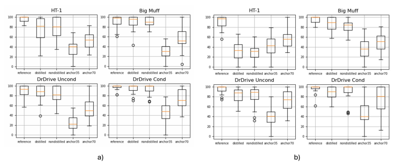
As presented in Figure 5, the listening test revealed that both distilled and non-distilled models scored quite high. This was good news, but it also meant that the perceptual advantage of distillation was not as pronounced as we anticipated. In fact, the finding suggests that it's still inconclusive whether there are any definitive perceptual advantages of distillation. This being said, we did notice a slight preference for distilled models in most cases. Non-distilled models also show greater variability, suggesting slightly less consistency in their perceived quality over their distilled counterparts.

Audio examples

Below are some audio examples from our attempts to model the DrDrive plugin with neural networks and optimization using KD. What you hear are three versions of the same audio where the only difference is what's creating the distortion effect.

DrDrive target - The target audio is taken straight out of the dataset. This is just the audio being recorded through the actual DrDrive plugin, sometimes referred to as the ground truth:

DrDrive student network (non-distilled) - Here, the audio is recorded through a small student network that is trained to mimicks the DrDrive distortion plugin. The network is trained on the regular dataset where the target audio came from:

DrDrive student network (distilled) - In this scenario, the audio is also recorded through a small student network that mimicks the DrDrive distortion plugin. However, instead of being trained on the regular dataset, this network has been "taught" by a larger teacher model:

For many more audio examples, visit the my dedicated GitHub repository.

Summary

In this post, I've tried to do a bit of what Roger once did for me; take something complex and slightly intimidating, and make it a little more approachable. We explored whether knowledge distillation, a technique built around the idea of good teacher-student combos, can help make neural audio distortion effects more efficient. We found that distillation can indeed improve performance for student models, effectively allowing us to shrink the networks while retaining accuracy. The results weren't perfectly uniform, dataset complexity, student size, and the gap between teacher and student all mattered, but the overall trend was clear. When applied thoughtfully, knowledge distillation is a promising tool for lightweight neural audio effects.

Our experiments showed consistent gains in many scenarios, especially with larger student models, while perceptual listening tests suggested a small but noticeable preference for distilled models. But just as importantly, our work raised new questions about how teachers should teach. Sometimes smaller, simpler teachers turned out to be better mentors than very large ones. This suggests that knowledge distillation is not a silver bullet, but it is a valuable addition to the toolbox for building real-time, deployable neural audio effects. Like most technologies riding the hypetrain, its real impact will likely be quieter, steadier, and more practical than dramatic, but that's often where the most meaningful progress lives.

Again, some useful links:

• Full AES research paper
• GitHub repository with source code and plugin/VST version of our distortion models.

For future work, more exhaustive architectural modifications should be considered. Additionally, designing more efficient loss functions could help refine the distance metrics between the probability distributions of teachers and students. Finally, employing a multiteacher ensemble approach could be advantageous in mitigating potential complexity gaps between models.

Sources

Fasciani, S., Simionato, R., and Tidemann, A., “A Universal Tool for Generating Datasets from Audio Effects,” in Proceedings of the Sound and Music Computing conference (SMC), 2024.

Hinton, G., Vinyals, O., and Dean, J., “Distilling the Knowledge in a Neural Network,” in NIPS Deep Learning and Representation Learning Workshop, 2015.

Simionato, R., Tidemann, A. "Compressing Neural Network Models of Audio Distortion Effects Using Knowledge Distillation Techniques." International Conference on Artificial Intelligence and Machine Learning for Audio (AES AIMLA), 2025.

Südholt, D., Wright, A., Erkut, C., and Välimäki, V., “Pruning Deep Neural Network Models of Guitar Distortion Effects,” IEEE/ACM Transactions on Audio, Speech, and Language Processing, 31, 2023, doi:10.1109/TASLP.2022.3223257.

Wright, A., Damskägg, E.-P., and Välimäki, V., “Real-Time Black-Box Modelling With Recurrent Neural Networks,” in Proceedings of the International Conference on Digital Audio Effects (DAFx), 2019.